Data Analysis

Is the number of people who hold college degrees significantly related to the amount of museums in their zip code?

# Count the number of museums per zip code
museum_count_per_zip <- museum_edu_df |>
  group_by(zip_code) |>
  summarize(n_museums = n())

# Merge the museum count back into the main dataset
museum_edu_df <- left_join(museum_edu_df, museum_count_per_zip, by = c("zip_code"), suffix = c(".museum_count_per_zip", ".museum_edu_df"))

# Linear regression: Number of Museums vs Highest Educational Attainment Category
regression_model_bach <- lm(bachelors ~ n_museums, data = museum_edu_df)

# Creating Regression Model Table
regression_model_bach |>
  broom::tidy() |>
  select(term, estimate, p.value) |>
  knitr::kable(digits=10)

term	estimate	p.value
(Intercept)	10.395863	0.000e+00
n_museums	0.171376	1.811e-07

E(bachelors) = β0 + β1(museum_n)

Intercept (Estimated Constant): The intercept is 10.39586. This is the estimated percentage of individuals with a bachelor’s degree when the number of museums (n_museums) is zero.

Coefficient for n_museums (Number of Museums): The coefficient for n_museums is 0.17138. This represents the estimated change in the percentage of individuals with a bachelor’s degree for each additional museum. The positive sign indicates a positive relationship, suggesting that, on average, as the number of museums increases, the percentage of individuals with a bachelor’s degree also tends to increase.

Statistical Significance: The associated p-value is very small (1.81e-07). This indicates that the number of museums is statistically significant in predicting the percentage of individuals with a bachelor’s degree.

In summary, the results suggest a statistically significant, positive relationship between the number of museums and the percentage of individuals with a bachelor’s degree.

Is median income a confounder on the relationship between educational attainment and the amount of museums?

Is the median income significantly related to the amount of museums in a zip code?

#Linear regression model: museums and medium income
regression_model_income <- lm(n_museums ~ median_income, data = museum_edu_df)

# Creating Regression Model Table
regression_model_income |>
  broom::tidy() |>
  select(term, estimate, p.value) |>
  knitr::kable(digits=10)

term	estimate	p.value
(Intercept)	2.537878269	0.00000e+00
median_income	-0.000014379	2.73268e-05

E(n_museums) = β0 + β1(median_income)

Intercept (Estimated Constant):

The intercept is 2.538. This is the predicted number of museums when the median income is zero.

Coefficient for median_income: The coefficient for median_income is -0.000014379. This represents the estimated change in number of museums for each unit change in income. The negative sign indicates a negative relationship, suggesting that, on average, as the number of median income increases, the number of museums tends to decrease.

Statistical Significance: The associated p-value is very small (2.73e-05). This indicates that the number of museums is statistically significant in predicting median income.

In summary, the results suggest a statistically significant,negative relationship between the median income and number of museums.

Is median income significantly related to the number of people who hold bachelor’s degrees?

#Linear regression model: college degrees and medium income
regression_model_bachincome <- lm(bachelors ~ median_income, data = museum_edu_df)

# Creating Regression Model Table
regression_model_bachincome |>
  broom::tidy() |>
  select(term, estimate, p.value) |>
  knitr::kable(digits=10)

term	estimate	p.value
(Intercept)	-6.7252860310	0
median_income	0.0004709779	0

E(bachelors) = β0 + β1(median_income)

Intercept (Estimated Constant):

The intercept is -6.725. This is the estimated percentage of individuals with a bachelor’s degree when the median income is zero.

Coefficient for median_income: The coefficient for median_income is 0.0004709779 This represents the estimated change in estimated percentage of individuals with a bachelor’s degree for each unit change in income. The positive sign indicates a positive relationship, suggesting that, on average, as the number of museums increases, the median income tends to increase

Statistical Significance: The associated p-value is very small (2.73e-05). This indicates that the median income is statistically significant in percentage of individual’s with a bachelor’s degrees.

In summary, the results suggest a statistically significant, positive relationship between the number of bachelor’s degrees and median income.

Regression model with both median income and number of museums

since median income is associated with both the number of museums and percentage of individuals with a bachelor’s degree, we should investigate if median income is a confounder between bachelor’s degrees and number of museums.

#linear regression model testing for confounding
model4 = lm(formula = bachelors ~ median_income + n_museums, data = museum_edu_df)

# Creating Regression Model Table
model4 |>
  broom::tidy() |>
  select(term, estimate, p.value) |>
  knitr::kable(digits=10)

term	estimate	p.value
(Intercept)	-7.3496990801	0
median_income	0.0004745601	0
n_museums	0.2448004363	0

E(bachelors) = β0 + β1(median_income) + β2(n_museums)

Intercept (Estimated Constant): The intercept is -7.350. This represents the estimated percentage of individuals with a bachelor’s degree when the number of museums (n_museums) is zero and median income (median_income) is zero.

Statistical significance: The p-values associated with each coefficient are very small (<2×10^−16), indicating that both median_income and n_museums are statistically significant predictors of the response variable.

Coefficient for n_museums: The coefficient for n_museums is 0.245. his represents the estimated change in the percentage of individuals with a bachelor’s degree for each additional museum, adjusted for median income. In the unadjusted model, the coefficient was: 0.17138. There is a 30% difference between the crude and unadjusted models, which is greater than 10%, signifying that income does infact confound the relationship between high educational attainment and amount of museums in a zipcode.

Comparison of models including income and excluding income

cv1_df = 
  crossv_mc(museum_edu_df, 100) 

cv1_df |> 
  mutate(
    mod_1  = map(train, \(df) lm(bachelors ~ n_museums, data = museum_edu_df)),
    mod_2  = map(train, \(df) lm(bachelors ~ median_income + n_museums, data = museum_edu_df))) |> 
  mutate(
    rmse_1 = map2_dbl(mod_1, test, \(mod, df) rmse(model = mod, data = df)),
    rmse_2 = map2_dbl(mod_2, test, \(mod, df) rmse(model = mod, data = df))) |>
  select(starts_with("rmse")) |>
  pivot_longer(
    everything(), names_to="model", values_to="rmse", names_prefix="rmse_") |>
  ggplot(aes(x=model, y=rmse)) + geom_violin()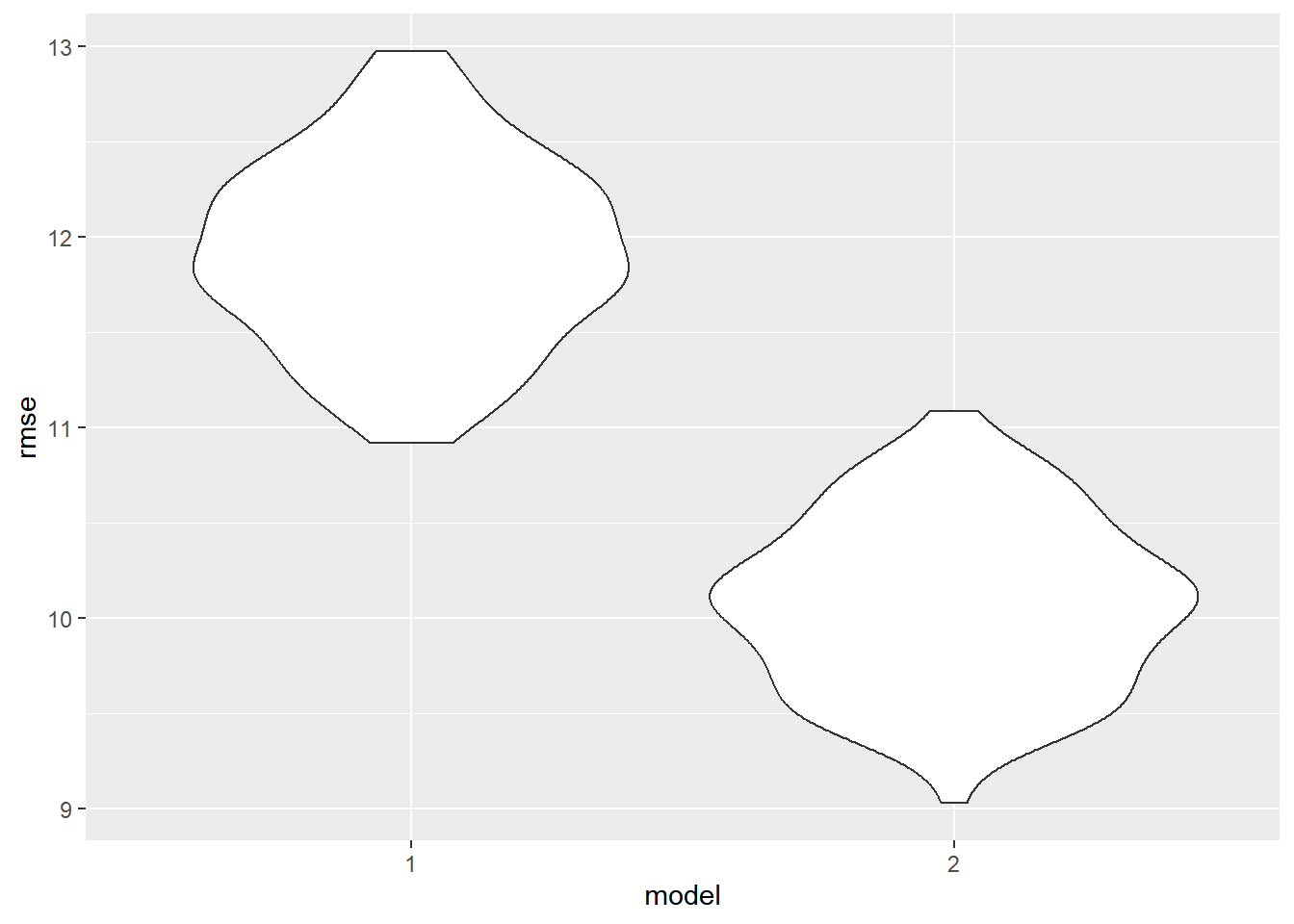

The model excluding income has a much higher root mean squared errors (RMSE) value than the model including income. This means that the model including income better fits our data.

Testing for Interaction between Median Income and Number of Museums

#linear regression model testing for confounding
model_int = lm(formula = bachelors ~ median_income + n_museums + median_income*n_museums, data = museum_edu_df)

# Creating Regression Model Table
model_int |>
  broom::tidy() |>
  select(term, estimate, p.value) |>
  knitr::kable(digits=10)

term	estimate	p.value
(Intercept)	-2.2849540454	6.528e-07
median_income	0.0002901590	0.000e+00
n_museums	-2.3996940174	0.000e+00
median_income:n_museums	0.0000986444	0.000e+00

E(bachelors) = β0 + β1(median_income) + β2(n_museums) + β3(median_income*n_museums)

The significant interaction term in the model implies that the effect of n_museums on bachelors is not constant across all levels of median_income. In other words, the relationship between the number of museums (n_museums) and the likelihood of having a bachelor’s degree (bachelors) is influenced by the level of median_income.

Comparison of income including models with and without interaction term:

cv2_df = 
  crossv_mc(museum_edu_df, 100) 

cv2_df |> 
  mutate(
    mod_1  = map(train, \(df) lm(formula = bachelors ~ median_income + n_museums + median_income*n_museums, data = museum_edu_df)),
    mod_2  = map(train, \(df) lm(formula = bachelors ~ median_income + n_museums, data = museum_edu_df))) |> 
  mutate(
    rmse_1 = map2_dbl(mod_1, test, \(mod, df) rmse(model = mod, data = df)),
    rmse_2 = map2_dbl(mod_2, test, \(mod, df) rmse(model = mod, data = df))) |>
  select(starts_with("rmse")) |>
  pivot_longer(
    everything(), names_to="model", values_to="rmse", names_prefix="rmse_") |>
  ggplot(aes(x=model, y=rmse)) + geom_violin()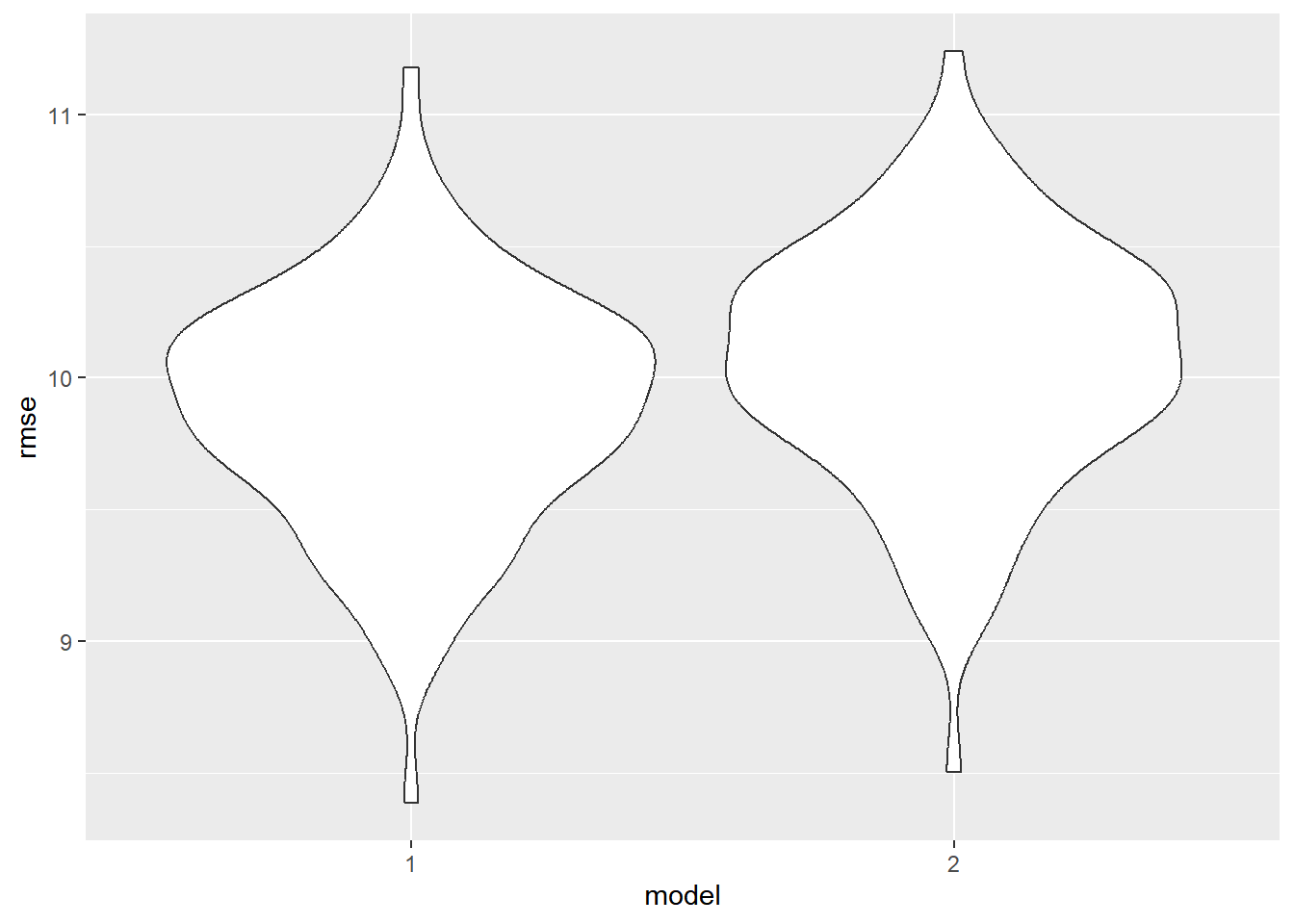

The model with an interaction term between bachelors and median income has a slightly lower RMSE value than the model without an interaction term. Ultimately, the model with interaction terms appears to be the best model.